 KHALM
KHALM
Deterministic anomaly detection
Neuromorphic One-class Vision Architecture
It learns what normal looks like.
Then it flags everything else — in 33 milliseconds.
One event camera, twenty minutes of routine driving, zero labels. KHALM-NOVA builds a memory of normal motion — per tile, per pattern — and from then on, anything unexpected drops its confidence score the moment it enters the frame. No GPU. No cloud. No guessing.
Raw events in. Confidence out.
Every 33 ms.
Real DSEC highway footage from a Prophesee event camera, played in real time. Left: the raw event stream — motion edges, nothing else. Right: the 16×12 tile aggregate the engine actually sees. Bottom: the SNN's confidence score. Watch it fall the moment an obstruction enters the window.
zurich_city_01_a, 34 seconds, real time. Green/red speckle (left) = ON/OFF events. Tile view (center-right) = the engine's input; red outlines mark tiles in burst condition. Timeline (bottom) = SNN winner drive — lower means more anomalous; shaded band = labeled obstruction; amber/red lines = P20/P30 alert thresholds. Clip: drive 259 → 196 as the anomaly enters.
The numbers, exactly as measured.
At 120 km/h, perception time is braking distance.
A vehicle at highway speed covers 33.3 metres per second. Perception latency stacks directly on top of the ~300 ms it takes physical brakes to pressurize. A hard 500 ms accumulation window would cost 16.7 metres before the decision even starts — so we slide the window instead: same statistics, one-tick response.
| System | Perception | Brake lag | Distance before braking |
|---|---|---|---|
| Surprised human driver | ~1500 ms | ~300 ms | ~60 m |
| Frame-based AEB (state of the art) | ~150 ms | ~300 ms | ~15 m |
| KHALM-NOVA, hard 500 ms window | 500 ms | ~300 ms | 26.6 m |
| KHALM-NOVA, sliding window @ 33 ms | 33 ms | ~300 ms | ~11 m |
Sliding the 500 ms window at every 33 ms tick keeps the statistical density the detector was trained on — measured AUROC parity with the non-overlapping window — while dropping worst-case perception latency 15×.
Three parts. No matrix math.
Encode
The event stream is binned into a 16×12 tile grid every 33 ms. Each tile becomes one byte: activity percentiles, span, flow — plus two reserved dark-line bits that stay off in healthy operation. A rolling 500 ms aggregate is re-encoded at every tick.
Learn normal
A spiking neural network with ternary (+1/0/−1) weights grows prototypes of normal driving via STDP-style plasticity — no backpropagation, no labels, no GPU. Twenty minutes of footage. Frozen once. Never retrains at deployment.
Score
Each tick, every prototype matches the encoded frame by popcount over ternary weights. The best match is the confidence drive. Novel patterns match nothing well → the drive drops → alert. Zero multiply-accumulate, start to finish.
Where it works — and where it's still research.
| Configuration | 01_a (19% obstr.) | 02_b (57% obstr.) | Combined (z) | Latency |
|---|---|---|---|---|
| Non-overlapping 500 ms window | 0.8385 | 0.5945 | 0.6405 | 500 ms |
| Sliding 500 ms @ 33 ms (shipping config) | 0.8445 | 0.5882 | 0.6355 | 33 ms |
| EMA aggregation, shift=4 (research variant) | 0.8511 | 0.5373 | 0.6092 | ~33 ms |
| Transducer baselines (no SNN, same encoding) | raw count 0.596 · tile z-score 0.613 | — | — | |
Known limitations, stated plainly
- Cross-scene generalization is unsolved. The same detector scores 0.845 within one clip and 0.588 within another; the combined figure requires per-clip z-score normalization. Multi-scene invariance is active research.
- 02_b-class obstructions are subtle. Slowly-developing or texture-like anomalies depress the drive weakly. Detection-rate vs. false-alarm trade-off is a deployment-time threshold choice.
- DSEC labels are sparse camera-frame samples (single 50 ms frames), not dense event-space ground truth. Numbers above are measured against them as-is.
- Benchmark scope: DSEC zurich_city driving clips, one event camera (Prophesee Gen4, left). Other domains need their own 20 minutes of normal.
Normal on the left. Novelty on the right.
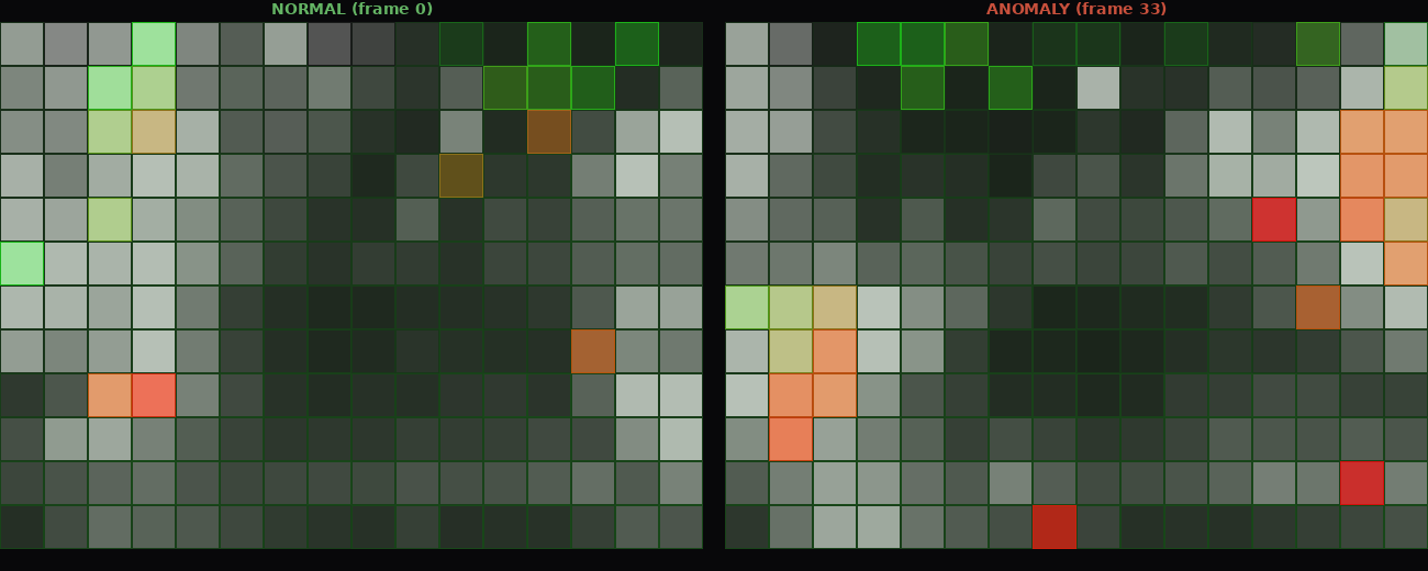
Each 40×40 pixel tile is colored by event density (greyscale) with a surprise overlay (green = matches learned normal, yellow = marginal, red = anomalous). Left: normal highway driving. Right: an obstruction event lights up novelty in the road-center and right-edge tiles.
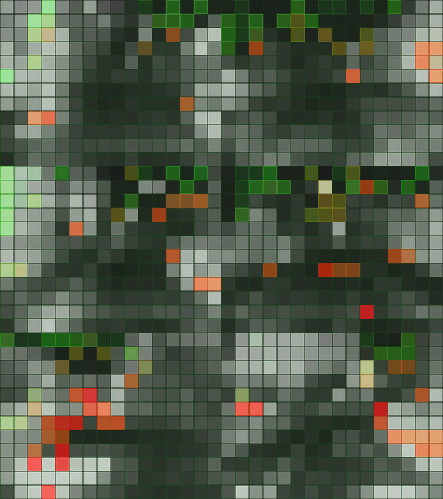
Animated novelty overlay over a 34-second highway sequence. Green tiles match the learned normal model; red tiles indicate unexpected patterns.
Building something that drives, flies, or watches?
If your system needs a deterministic second opinion that costs a milliwatt and never bluffs — let's talk.